4 Multiple regression

4.1 Introductory examples

Setup: response variable \(y\), predictors \(x_1\), \(x_2\), …, \(x_k\).

4.1.1 Example 1: Fuel Use

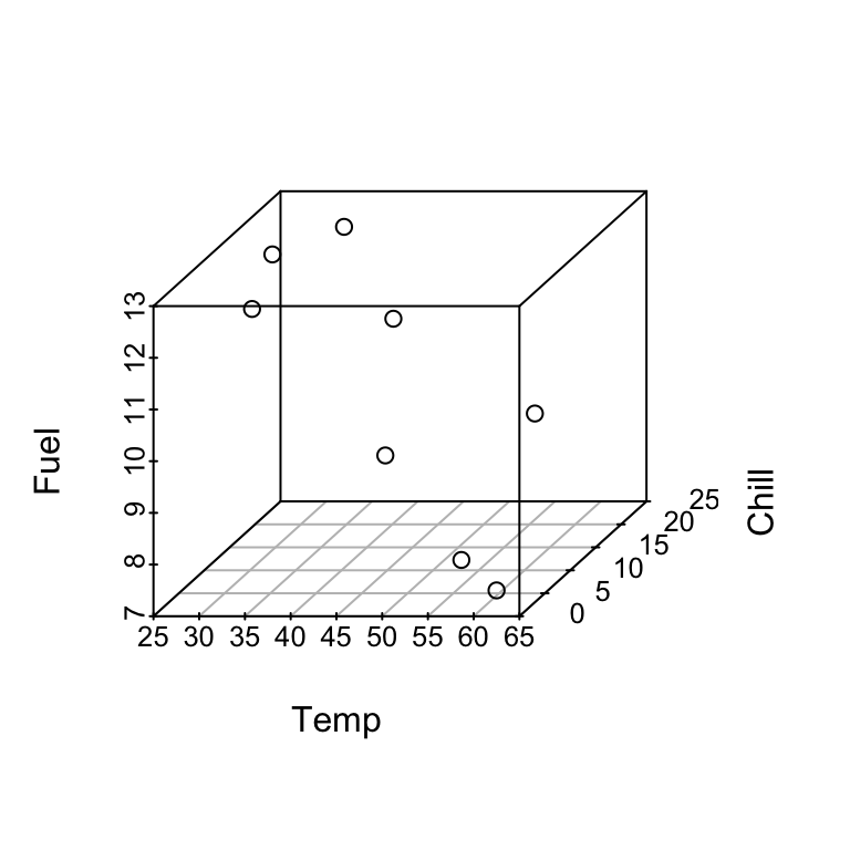
Example from Section 2. Information was recorded on fuel usage and average temperature (\(^oF\)) over the course of one week for eight office complexes of similar size. Data are from Bowerman and Schafer (1990).

\(y\) = fuel use,

\(x_1\) = temperature,

\(x_2\) = chill index.

Data:

Temp	Fuel	Chill
28.0	12.4	18
28.0	11.7	14
32.5	12.4	24
39.0	10.8	22
45.9	9.4	8
57.8	9.5	16
58.1	8.0	1
62.5	7.5	0

We wish to use \(x_1\) and \(x_2\) to predict \(y\). This should give more accurate predictions than either \(x_1\) or \(x_2\) alone.

A multiple linear regression model is: fuel use \(\approx\) a linear function of temperature and chill index.

More precisely:

\[y = \beta_0 + \beta_1 x_1 + \beta_2 x_2 + \epsilon.\]

As before, \(\epsilon\) is the unobserved error, \(\beta_0, \beta_1, \beta_2\) are the unknown parameters.

When \(\mathbb{E}[\epsilon ] = 0\) we have

\[\mathbb{E}[y] = \beta_0 + \beta_1 x_1 + \beta_2 x_2.\]

In SLR we can check model appropriateness by plotting \(y\) vs \(x\) and observing whether the points fall close to a line. Here we could construct a 3-d plot of \(y\), \(x_1\), \(x_2\) and points should fall close to a plane.

For a given set of values of \(x_1\) and \(x_2\), say \(x_1 = 45.9\) and \(x_2 = 8\), the model says that the mean fuel use is:

\[\mathbb{E}[y] = \beta_0 + \beta_1 \times 45.9 + \beta_2 \times 8.\]

If \(x_1 = x_2 = 0\) then \(\mathbb{E}[y] = \beta_0\), the model intercept.

To interpret \(\beta_1\) suppose \(x_1 = t\) and \(x_2 = c\). Then

\[\mathbb{E}[y]=\beta_0 + \beta_1 \times t + \beta_2 \times c.\]

Now suppose \(x_1\) increases by \(1\) and \(x_2\) stays fixed:

\[\mathbb{E}[y]=\beta_0 + \beta_1 \times (t + 1) + \beta_2 \times c.\]

Substracting these we find that \(\beta_1\) is the increase in \(\mathbb{E}[y]\) associated with 1 unit increase in \(x_1\) for a fixed \(x_2\).

I.e. two weeks having the same chill index but whose temperature differed by \(1^o\) would have a mean fuel use difference of \(\beta_1\).

4.1.2 Example 2: Categorical predictors

Suppose we wish to predict the fuel efficiency of different car types. Data are from Cryer and Miller (1991). We have data on:

\(y\) = gallons per mile (gpm),

\(x_1\) = car weight (w),

\(x_2\) = transmission type (ttype): 1 = automatic or 0 = manual.

We use the model

\[\mathbb{E}[y] = \beta_0 + \beta_1 x_1 + \beta_2 x_2.\]

\(\beta_0\) = the mean gpm for cars of weight \(w = 0\) and ttype = manual. \(\beta_1\) = change in mean gpm when weight increases by 1 for the same ttype. \(\beta_2\) = change in mean gpm when the car of the same weight is changed from manual to automatic.

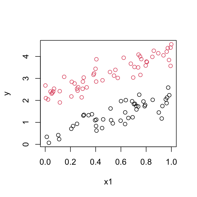
The model says that:

\[\begin{align*} \mathbb{E}[y] & = \beta_0 + \beta_1 x_1 \quad \mbox{ for manual}\\ & = \beta_0 + \beta_2 + \beta_1 x_1 \quad \mbox{ for automatic.} \end{align*}\]

Therefore we are fitting two lines with different intercepts but the same slope.

The data should look like:

Suppose the data look like this:

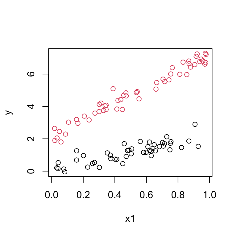
This suggests we should fit two lines with different intercepts and different slopes. We introduce a third predictor:

\[\mathbb{E}[y] = \beta_0 + \beta_1 x_1 + \beta_2 x_2 + \beta_3 x_1x_2,\]

giving:

\[\begin{align*} \mathbb{E}[y] & = \beta_0 + \beta_1 x_1 \quad \mbox{ for manual}\\ & = (\beta_0 + \beta_2) + (\beta_1 + \beta_3) x_1 \quad \mbox{ for automatic.} \end{align*}\]

The term \(x_1x_2\) is called an interaction term.

Here:

\(\beta_2\) = difference in intercept

\(\beta_3\) = difference in slope.

4.1.3 Example 3: Polynomials

We have one predictor \(x\) but the plot of \(y\) vs \(x\) exhibits a quadratic pattern.

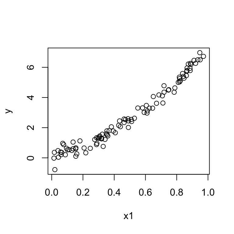Then we can fit a multiple regression model:

\[\mathbb{E}[y] = \beta_0 + \beta_1 x + \beta_2 x^2.\]

This is also called a quadratic regression model or, more generally, a polynomial regression model.

Higher order polynomial regression models can also be used if needed.

Link: http://www.rpubs.com/kdomijan/333155

4.1.4 Example 4: Nonlinear relationships

For example,

\[y = \alpha x_1 ^{\beta x_2} \epsilon.\]

Nonlinear models can sometimes be linearized, for example:

\[log(y) = log(\alpha) + \beta x_2 log(x_1) + log(\epsilon).\]

Here: \(x = x_2 log(x_1)\).

NOTE: the term linear refers to the linearity of regression parameters.

A general form for multiple linear regression model (with two explanatory variables):

\[y = \beta_0 f_0(x_1, x_2) + \beta_1 f_1(x_1, x_2) + \beta_2 f_2(x_1, x_2) + \dots\]

where \(f_j(x_1, x_2)\) are known functions of explanatory variables.

The extension to more than two explanatory variables is straightforward.

4.1.5 Diamonds data

diamonds |> ggplot(aes(x = carat, y = log(price), col = color)) + geom_point() +
  facet_wrap(~clarity)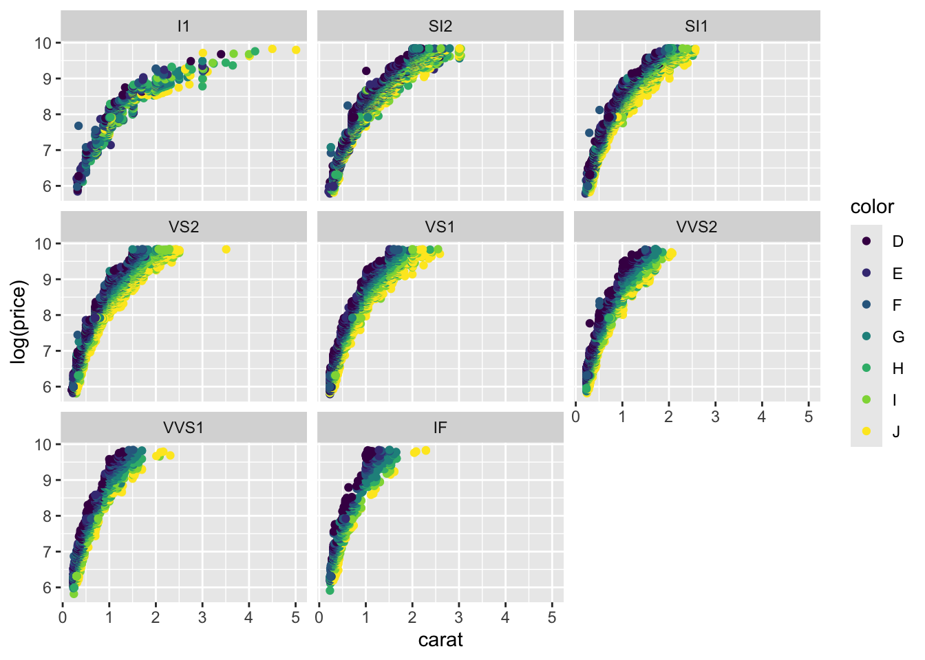

# model.orig <- lm(log(price) ~ poly(carat,2) + color + clarity +cut,  diamonds)
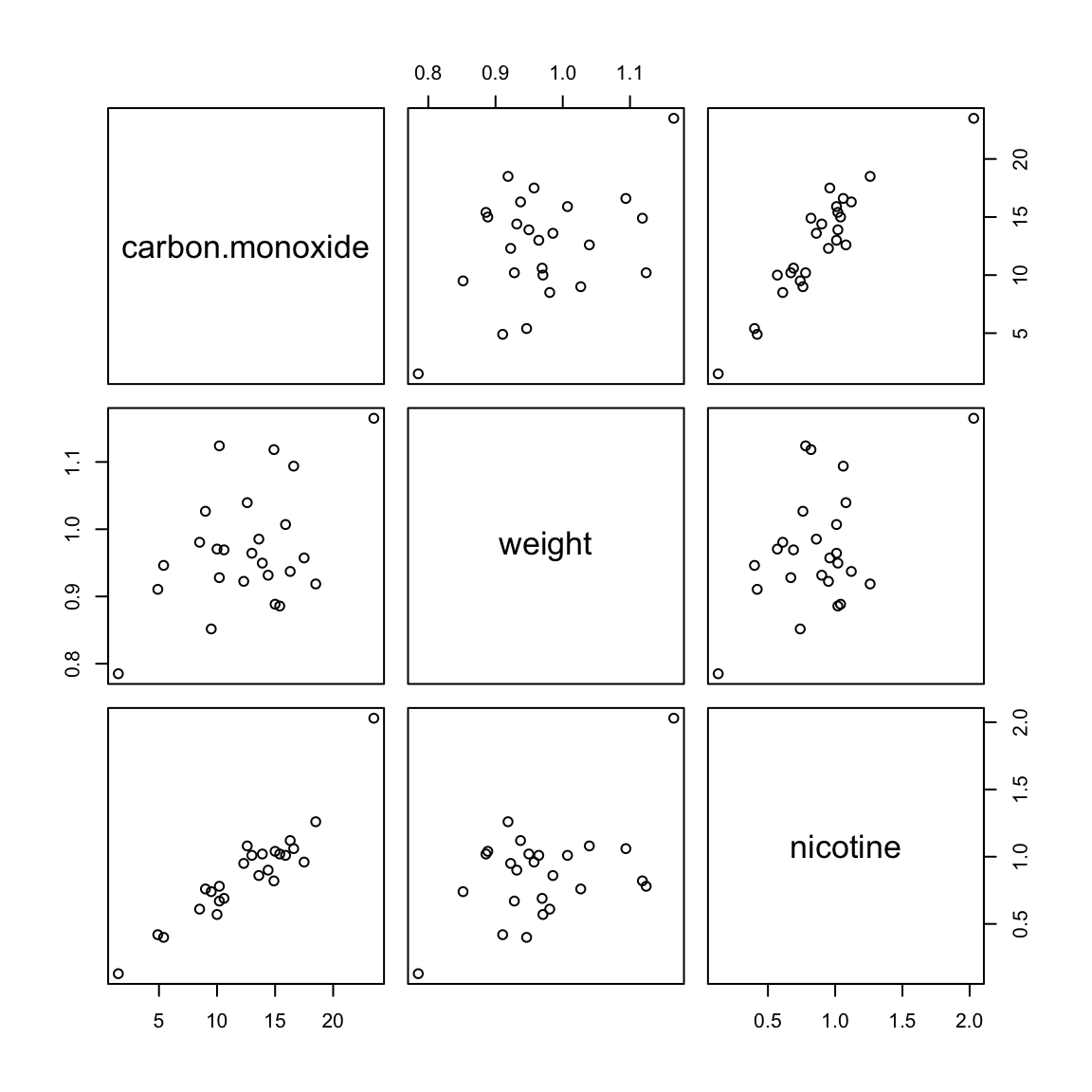
# summary(model.orig)

4.1.6 Cigarette Data continued

Data from 3.7.4. Consider a second predictor (weight):

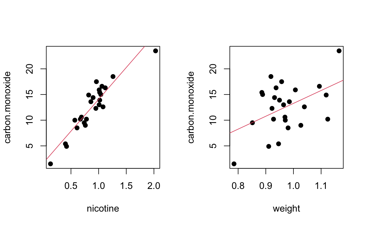
Regression (nicotine only)

summary(fit)

## 
## Call:
## lm(formula = carbon.monoxide ~ nicotine)
## 
## Residuals:
##     Min      1Q  Median      3Q     Max 
## -3.3273 -1.2228  0.2304  1.2700  3.9357 
## 
## Coefficients:
##             Estimate Std. Error t value Pr(>|t|)    
## (Intercept)   1.6647     0.9936   1.675    0.107    
## nicotine     12.3954     1.0542  11.759 3.31e-11 ***
## ---
## Signif. codes:  0 '***' 0.001 '**' 0.01 '*' 0.05 '.' 0.1 ' ' 1
## 
## Residual standard error: 1.828 on 23 degrees of freedom
## Multiple R-squared:  0.8574, Adjusted R-squared:  0.8512 
## F-statistic: 138.3 on 1 and 23 DF,  p-value: 3.312e-11

Regression (weight only)

summary(fit2)

## 
## Call:
## lm(formula = carbon.monoxide ~ weight)
## 
## Residuals:
##    Min     1Q Median     3Q    Max 
## -6.524 -2.533  0.622  2.842  7.268 
## 
## Coefficients:
##             Estimate Std. Error t value Pr(>|t|)  
## (Intercept)  -11.795      9.722  -1.213   0.2373  
## weight        25.068      9.980   2.512   0.0195 *
## ---
## Signif. codes:  0 '***' 0.001 '**' 0.01 '*' 0.05 '.' 0.1 ' ' 1
## 
## Residual standard error: 4.289 on 23 degrees of freedom
## Multiple R-squared:  0.2153, Adjusted R-squared:  0.1811 
## F-statistic: 6.309 on 1 and 23 DF,  p-value: 0.01948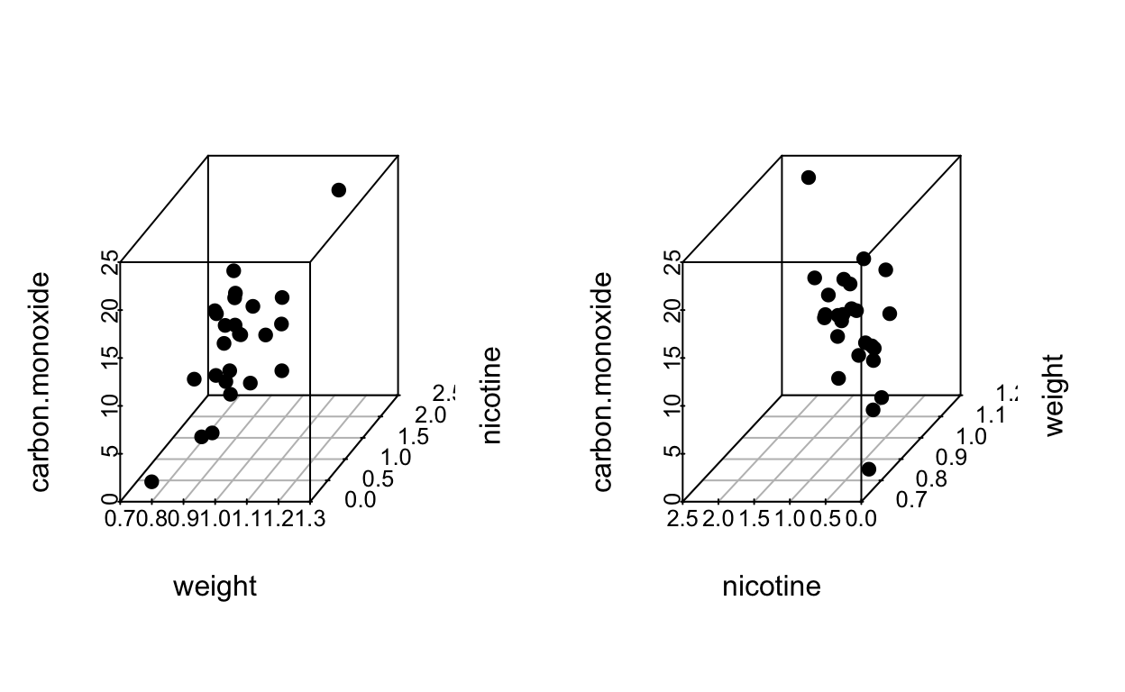

Regression (both predictors)

fit3 <- lm(carbon.monoxide ~ weight + nicotine)
summary(fit3)

## 
## Call:
## lm(formula = carbon.monoxide ~ weight + nicotine)
## 
## Residuals:
##     Min      1Q  Median      3Q     Max 
## -3.3304 -1.2249  0.2314  1.2677  3.9371 
## 
## Coefficients:
##             Estimate Std. Error t value Pr(>|t|)    
## (Intercept)  1.61398    4.44663   0.363    0.720    
## weight       0.05883    5.02395   0.012    0.991    
## nicotine    12.38812    1.24473   9.952 1.32e-09 ***
## ---
## Signif. codes:  0 '***' 0.001 '**' 0.01 '*' 0.05 '.' 0.1 ' ' 1
## 
## Residual standard error: 1.87 on 22 degrees of freedom
## Multiple R-squared:  0.8574, Adjusted R-squared:  0.8444 
## F-statistic: 66.13 on 2 and 22 DF,  p-value: 4.966e-10

Regression (quadratic)

nicotine.sq <- nicotine^2
fit4 <- lm(carbon.monoxide ~ nicotine + nicotine.sq)
summary(fit4)

## 
## Call:
## lm(formula = carbon.monoxide ~ nicotine + nicotine.sq)
## 
## Residuals:
##     Min      1Q  Median      3Q     Max 
## -2.9857 -1.1052  0.1834  0.8654  3.4145 
## 
## Coefficients:
##             Estimate Std. Error t value Pr(>|t|)    
## (Intercept)   -1.784      1.453  -1.227  0.23264    
## nicotine      20.111      2.775   7.248 2.92e-07 ***
## nicotine.sq   -3.730      1.267  -2.945  0.00749 ** 
## ---
## Signif. codes:  0 '***' 0.001 '**' 0.01 '*' 0.05 '.' 0.1 ' ' 1
## 
## Residual standard error: 1.583 on 22 degrees of freedom
## Multiple R-squared:  0.8977, Adjusted R-squared:  0.8884 
## F-statistic: 96.53 on 2 and 22 DF,  p-value: 1.284e-11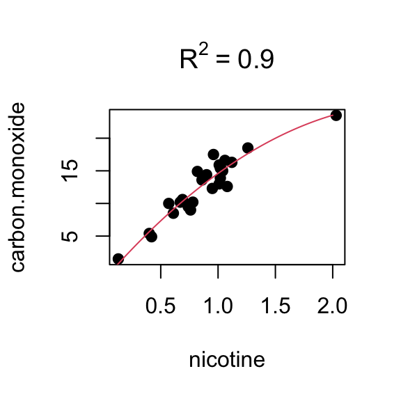

4.2 Least squares estimation for multiple regression

Our model states that:

\[y = \beta_0 + \beta_1x_{1} + \beta_2x_{2} + ... + \beta_kx_k + \epsilon,\]

where \(k<n\).

For each observation we have:

\[y_i = \beta_0 + \beta_1x_{i1} + \beta_2x_{i2} + ... + \beta_kx_{ik} + \epsilon_i.\]

We can write this more compactly using matrix notation.

Let \(\mathbf{Y}\) be the response vector:

\[\mathbf{Y} =\begin{bmatrix} y_{1} \\ y_{2} \\ \vdots\\ y_{n} \end{bmatrix}\]

Let \(\mathbf{X}\) be the \(n \times p\) matrix, where \(p = k+1\):

\[\mathbf{X} = \begin{bmatrix} 1 & x_{11} & x_{12} & x_{13} & \dots & x_{1k} \\ 1 & x_{21} & x_{22} & x_{23} & \dots & x_{2k} \\ \vdots & \vdots & \vdots & \vdots & \ddots & \vdots \\ 1 & x_{n1} & x_{n2} & x_{n3} & \dots & x_{nk} \end{bmatrix}\]

Let \(\boldsymbol{\beta}\) be the \(p\)-dim parameter vector:

\[\boldsymbol{\beta} =\begin{bmatrix} \beta_{0} \\ \beta_{1} \\ \vdots\\ \beta_{k} \end{bmatrix}\]

Let \(\boldsymbol{\epsilon}\) be the \(n\)-dim error vector:

\[\boldsymbol{\epsilon} =\begin{bmatrix} \epsilon_{1} \\ \epsilon_{2} \\ \vdots\\ \epsilon_{n} \end{bmatrix}\]

The model states that:

\[\mathbf{Y}=\mathbf{X}\boldsymbol{\beta} + \boldsymbol{\epsilon}.\]

The vector of fitted values is:

\[\hat{\mathbf{Y}}=\mathbf{X}\hat{\boldsymbol{\beta}}.\]

The corresponding residual values are:

\[\mathbf{e}=\mathbf{Y}-\hat{\mathbf{Y}}.\]

The OLS estimates minimise:

\[S(\boldsymbol{\beta}) = \sum_{i=1}^{n}(y_i-\beta_0-\beta_1x_{i1}- ... - \beta_kx_{ik})^2\]

over \(\boldsymbol{\beta}\).

Therefore the OLS estimates satisfy:

\[\frac{\delta S(\boldsymbol{\beta})}{\delta \beta_j} = 0, \quad \forall j\]

and as before we evaluate at \(\hat{\boldsymbol{\beta}}\)

\[\frac{\delta S(\boldsymbol{\beta})}{\delta \beta_0} = -2 \sum_{i=1}^{n}(y_i-\beta_0-\beta_1x_{i1}- ... - \beta_kx_{ik})\]

\[\frac{\delta S(\boldsymbol{\beta})}{\delta \beta_j} = -2 \sum_{i=1}^{n} x_{ij}(y_i-\beta_0-\beta_1x_{i1}- ... - \beta_kx_{ik}), \quad \forall j = 1,...,k.\]

The OLS estimates of \(\boldsymbol{\beta}\) satisfy:

\[\sum_{i=1}^{n}(y_i-\hat{\beta}_0-\hat{\beta}_1x_{i1}- ... - \hat{\beta}_kx_{ik}) = 0\]

and

\[\sum_{i=1}^{n}(y_i-\hat{\beta}_0-\hat{\beta}_1x_{i1}- ... - \hat{\beta}_kx_{ik})x_{ij} = 0, \quad \forall j = 1,...,k.\]

These normal equations (see (3.1) and (3.2)) can be written as:

\[\sum_{i=1}^{n}e_i = 0\]

and

\[\sum_{i=1}^{n}x_{ij}e_i = 0, \quad \forall j = 1,...,k.\]

We can combine this into one matrix equation:

\[\mathbf{X}^T\mathbf{e}= \mathbf{0}\]

or equivalently:

\[\mathbf{X}^T(\mathbf{Y} - \mathbf{X}\hat{\boldsymbol{\beta}})= \mathbf{0}\]

Therefore the OLS estimator \(\hat{\boldsymbol{\beta}}\) satisfies:

\[\begin{align} \mathbf{X}^T\mathbf{X}\hat{\boldsymbol{\beta}} &= \mathbf{X}^T\mathbf{Y}\\ \hat{\boldsymbol{\beta}} &= (\mathbf{X}^T\mathbf{X})^{-1} \mathbf{X}^T\mathbf{Y}.\tag{4.1} \end{align}\]

Matrix \(\mathbf{X}^T\mathbf{X}\) is non-singular (i.e has an inverse) iff \(rank(\mathbf{X}) =p\), i.e. \(\mathbf{X}\) has full rank and the columns of \(\mathbf{X}\) are linearly independent.

4.2.1 Estimation of \(\sigma^2\) = Var\((\epsilon)\)

A point estimate of \(\sigma^2\) is the mean squared error:

\[\hat{\sigma}^2 = \mbox{MSE} = \frac{\mbox{SSE}}{n-p} = \frac{\sum_{i=1}^n e_i^2}{n-p}.\]

4.2.2 Estimation of Var\((\hat{\beta})\)

\[\mbox{Var}(\hat{\boldsymbol{\beta}}) = (\mathbf{X}^T\mathbf{X})^{-1} \sigma^2.\]

\[\widehat{\mbox{Var}(\hat{\boldsymbol{\beta}})} = (\mathbf{X}^T\mathbf{X})^{-1} \hat{\sigma}^2.\]

4.3 Prediction from multiple linear regression model

As we have seen already, to predict from a multiple regression model we use:

\[\hat{y}_i = \hat{\beta}_0+ \hat{\beta}_1x_{i1}+ \cdots+\hat{\beta}_kx_{ik}\]

or \[\hat{\mathbf{Y}} = \mathbf{X}\hat{\boldsymbol{\beta}}\]

At a particular set of \(x_0\) values we predict the response \(y_0\) by:

\[\hat{y}_0 = \mathbf{x}_0^T\hat{\boldsymbol{\beta}}\]

where \(\mathbf{x}_0^T = ( 1, x_{01},x_{02},..., x_{0k})\).

We also use \(\hat{y}_0\) to estimate \(\mathbb{E}(y_0)\), the mean of \(y_0\) at a given set of \(x_0\) values.

The \(\mbox{S.E.}\) for the estimate of the mean \(\mathbb{E}(y_0)\) is:

\[\mbox{S.E.}_{\mbox{fit}} (\hat{y}_0)= \hat{\sigma}\sqrt{\mathbf{x}_0^T(\mathbf{X}^T\mathbf{X})^{-1}\mathbf{x}_0}.\]

A \(1-\alpha\) confidence interval for the expected response at \(\mathbf{x}_0\) is given by:

\[\hat{y}_0 \pm t_{n-p}(\alpha/2) \times \mbox{S.E.}_{\mbox{fit}} (\hat{y}_0).\]

The \(\mbox{S.E.}\) for the predicted \(y_0\):

\[\mbox{S.E.}_{\mbox{pred}}(\hat{y}_0) = \hat{\sigma}\sqrt{1+ \mathbf{x}_0^T(\mathbf{X}^T\mathbf{X})^{-1}\mathbf{x}_0}.\]

Note: \[\mbox{S.E.}_{\mbox{pred}}(\hat{y}_0)= \sqrt{\hat{\sigma}^2+\mbox{S.E.}_{\mbox{fit}}(\hat{y}_0)^2}\]

4.4 Regression models in matrix notation: examples

4.4.1 Example 1: SLR

The \(\mathbf{X}\) matrix is:

\[\mathbf{X} = \begin{bmatrix} 1 & x_{1}\\ \vdots & \vdots\\ 1 &x_{n} \end{bmatrix}\]

To estimate the coefficients \(\hat{\boldsymbol{\beta}}\):

\[\begin{align*} \mathbf{X}^T\mathbf{X} &= \begin{bmatrix} n & \sum x_{i}\\ \sum x_{i}& \sum x_{i}^2 \end{bmatrix}\\ (\mathbf{X}^T\mathbf{X})^{-1} & = \frac{1}{n \sum x_{i}^2 - (\sum x_{i})^2}\begin{bmatrix} \sum x_{i}^2& -\sum x_{i}\\ -\sum x_{i} & n \end{bmatrix} \\ & = \frac{1}{n (\sum x_{i}^2 - n\bar{x}^2)}\begin{bmatrix} \sum x_{i}^2 & -n\bar{x} \\ -n\bar{x} & n \end{bmatrix} \\ & = \frac{1}{S_{xx}}\begin{bmatrix} \sum x_{i}^2/n & -\bar{x} \\ -\bar{x} & 1 \end{bmatrix} \\ \mathbf{X}^T\mathbf{Y} &= \begin{bmatrix} \sum y_{i} \\ \sum x_{i}y_{i} \end{bmatrix} = \begin{bmatrix} n\bar{y} \\ \sum x_{i}y_{i} \end{bmatrix}\\ \hat{\boldsymbol{\beta}} & = (\mathbf{X}^T\mathbf{X})^{-1}\mathbf{X}^T\mathbf{Y} \\ & = \frac{1}{S_{xx}}\begin{bmatrix} \bar{y}\sum x_{i}^2 -\bar{x} \sum x_{i}y_i \\ -n \bar{x} \bar{y} + \sum x_{i}y_i \end{bmatrix} \end{align*}\]

With some algebra, this gives:

\[\hat{\beta}_1 = \frac{S_{xy}}{S_{xx}}\] and

\[\hat{\beta}_0= \bar{y} - \hat{\beta}_1\bar{x}\]

as before, and

\[\begin{align*} \mbox{Var}(\hat{\boldsymbol{\beta}})& = (\mathbf{X}^T\mathbf{X})^{-1}\sigma^2\\ & = \frac{\sigma^2}{S_{xx}} \begin{bmatrix} \sum x_{i}^2/n& -\bar{x} \\ -\bar{x}& 1 \end{bmatrix} \end{align*}\]

which gives

\[\mbox{Var}(\hat{\beta}_0) = \sigma^2\left(\frac{1}{n}+ \frac{\bar{x}^2}{S_{xx}}\right),\]

\[\mbox{Var}(\hat{\beta}_1) = \frac{\sigma^2}{S_{xx}},\]

\[\mbox{Cov}(\hat{\beta}_0, \hat{\beta}_1) = -\bar{x}\frac{\sigma^2}{S_{xx}}.\]

4.4.2 Example 2

Example from Stapleton (2009), Problem 3.1.1, pg 81.

A scale has 2 pans. The measurement given by the scale is the difference between the weight in pan 1 and pan 2, plus a random error \(\epsilon\).

Suppose that \(\mathbb{E}[\epsilon] = 0\) and \(\mbox{Var}(\epsilon) = \sigma^2\) and the \(\epsilon_i\) are independent.

Suppose also that two objects have weight \(\beta_1\) and \(\beta_2\) and that 4 measurements are taken:

Pan 1: object 1, Pan 2: empty
Pan 1: empty, Pan 2: object 2
Pan 1: object 1, Pan 2: object 2
Pan 1: object 1 and 2, Pan 2: empty

Let \(y_1\), \(y_2\), \(y_3\) and \(y_4\) be the four observations. Then:

\[\begin{align*} y_1 & = \beta_1 + \epsilon_1\\ y_2 & =- \beta_2 + \epsilon_2\\ y_3 & = \beta_1 - \beta_2 + \epsilon_3\\ y_4 & = \beta_1 + \beta_2 + \epsilon_4\\ \end{align*}\]

\(\mathbf{X} = \begin{bmatrix} 1 &0 \\ 0 & -1 \\ 1 & -1 \\ 1 & 1 \end{bmatrix}\)

\(\mathbf{Y} = \begin{bmatrix} y_1 \\ y_2 \\ y_3 \\ y_4 \end{bmatrix}\)

\(\boldsymbol{\beta} = \begin{bmatrix} \beta_1 \\ \beta_2 \end{bmatrix}\)

\(\boldsymbol{\epsilon} = \begin{bmatrix} \epsilon_1 \\ \epsilon_2 \\ \epsilon_3 \\ \epsilon_4 \end{bmatrix}\)

The model is:

\[\mathbf{Y} = \begin{bmatrix} 1 &0 \\ 0 & -1 \\ 1 & -1 \\ 1 & 1 \end{bmatrix} \times\begin{bmatrix} \beta_1 \\ \beta_2 \end{bmatrix} + \boldsymbol{\epsilon} = \mathbf{X}\boldsymbol{\beta} + \boldsymbol{\epsilon}\]

The OLS estimates of \(\boldsymbol{\beta}\) are given by:

\[\hat{\boldsymbol{\beta}} = (\mathbf{X}^T\mathbf{X})^{-1} \mathbf{X}^T\mathbf{Y}.\]

\[\begin{align*} \mathbf{X}^T\mathbf{X} & = \begin{bmatrix} 1 & 0 & 1 & 1\\ 0 & -1 & -1 & 1\\ \end{bmatrix} \begin{bmatrix} 1 & 0 \\ 0 & -1 \\ 1 & -1 \\ 1 & 1\\ \end{bmatrix}\\ & = \begin{bmatrix} 3 & 0 \\ 0 & 3 \\ \end{bmatrix}\\ & = 3\begin{bmatrix} 1 & 0 \\ 0 & 1 \\ \end{bmatrix}\\ \mathbf{X}^T\mathbf{Y} &= \begin{bmatrix} y_1 + y_3 + y_4\\ -y_2 - y_3 + y_4\\ \end{bmatrix}\\ \hat{\boldsymbol{\beta}} & = (\mathbf{X}^T\mathbf{X})^{-1} \mathbf{X}^T\mathbf{Y}\\ & = \frac{1}{3}\begin{bmatrix} 1 & 0 \\ 0 & 1 \\ \end{bmatrix} \begin{bmatrix} y_1 + y_3 + y_4\\ -y_2 - y_3 + y_4\\ \end{bmatrix}\\ & = \frac{1}{3}\begin{bmatrix} y_1 + y_3 + y_4\\ -y_2 - y_3 + y_4\\ \end{bmatrix}\\ \mbox{Var}(\hat{\boldsymbol{\beta}}) &= (\mathbf{X}^T\mathbf{X})^{-1} \sigma^2 = \frac{1}{3}\begin{bmatrix} 1 & 0 \\ 0 & 1 \\ \end{bmatrix} \sigma^2.\\ \end{align*}\]

Can we improve the experiment so that the 4 measurements yield estimates of \(\boldsymbol{\beta}\) with smaller variance?

present design: \(\mbox{Var}(\hat{\beta}_i) = \frac{\sigma^2}{3}\)
Let \(\mathbf{X} = \begin{bmatrix} 1 & -1 \\ 1 & -1 \\ 1 & 1 \\ 1 & 1 \end{bmatrix}\),

\(\mbox{Var}(\hat{\beta}_i) = \frac{\sigma^2}{4}\)

Let \(\mathbf{X} = \begin{bmatrix} 1 & 0 \\ 1 & 0 \\ 0 & 1 \\ 0 & 1 \end{bmatrix}\),

\(\mbox{Var}(\hat{\beta}_i) = \frac{\sigma^2}{2}\).

4.5 The formal multiple regression model and properties

4.5.1 Concepts: random vectors, covariance matrix, multivariate normal distribution (MVN).

Let \(Y_1,...,Y_n\) be r.v.s defined on a common probability space.

Then \(\mathbf{Y}\) is a random vector.

Let \(\mu_i = \mathbb{E}[y_i]\) and \(\boldsymbol{\mu} = \begin{bmatrix} \mu_1 \\ \vdots \\ \mu_n \end{bmatrix}\).

Then \(\boldsymbol{\mu}\) is a mean vector and we write:

\[\mathbb{E}[\mathbf{Y}] = \boldsymbol{\mu}.\]

Let \(\sigma_{ij} = Cov(y_i, y_j)\). Then \(\boldsymbol{\Sigma}\) is the covariance matrix of \(\mathbf{Y}\), where \(\boldsymbol{\Sigma}_{ij} = [\sigma_{ij}].\)

We write:

\[\mbox{Var}(\mathbf{Y}) = \boldsymbol{\Sigma}.\]

Aside:

\(\mbox{Cov}(Y_i,Y_j) = \mathbb{E}[(Y_i-\mathbb{E}[Y_i])(Y_j-\mathbb{E}[Y_j])]\)

\(\mbox{Cov}(Y_i,Y_i) = \mbox{Var}(Y_i)\)

If \(Y_i,Y_j\) are independent then \(\mbox{Cov}(Y_i,Y_j) = 0\).

When \(Y_i,Y_j\) have bivariate normal distribution, if \(\mbox{Cov}(Y_i,Y_j) = 0\), then \(Y_i,Y_j\) are independent.

Fact: Suppose \(\mathbf{Y}\) has mean \(\boldsymbol{\mu}\) and variance \(\boldsymbol{\Sigma}\). Then for a vector of constants \(\mathbf{b}\) and matrix of constants \(\mathbf{C}\):

\[\mathbb{E}[\mathbf{C}\mathbf{Y} + \mathbf{b}] = \mathbf{C}\boldsymbol{\mu} + \mathbf{b}\]

and

\[\mbox{Var}( \mathbf{C}\mathbf{Y} + \mathbf{b} ) = \mathbf{C}\boldsymbol{\Sigma} \mathbf{C}^T.\]

Defn: A random \(n\) - dim vector \(\mathbf{Y}\) is said to have a MVN distribution if \(\mathbf{Y}\) can be written as \[\mathbf{Y} = \mathbf{A}\mathbf{Z} + \boldsymbol{\mu}\] where:

\(Z_1, Z_2, ..., Z_p\) are iid N(0,1),
\(\mathbf{A}\) is an \(n \times p\) matrix of constants and
\(\boldsymbol{\mu}\) is an \(n\) vector of constants.

Notes:

Random vector \(\mathbf{Z}\) is multivariate normal with mean \(\mathbf{0}\) and covariance \(\mathbf{I}_p\) since \(Z_i\)s are independent so their covariances are 0. We write: \[\mathbf{Z} \sim N_p(\mathbf{0}, \mathbf{I}_p).\]
\(\mathbb{E}[\mathbf{Y}] = \mathbb{E}[\mathbf{A}\mathbf{Z} + \boldsymbol{\mu}] = \boldsymbol{\mu}\),
\(\mbox{Var}(\mathbf{Y}) = \mathbf{A}\mathbf{A}^T\),
\(\mathbf{Y} \sim N_n (\boldsymbol{\mu}, \mathbf{A}\mathbf{A}^T)\).

4.5.2 Multiple regression model

\[\mathbf{Y}=\mathbf{X}\boldsymbol{\beta} + \boldsymbol{\epsilon}.\]

\(\mathbf{Y}=\) \(n\) - dimensional response random vector.

\(\boldsymbol{\beta}=\) unknown \(p\) - dimensional parameter vector.

\(\mathbf{X}=\) an \(n \times p\) matrix of constants.

\(\boldsymbol{\epsilon}=\) \(n\) - dimensional error vector.

Assumptions:

Linearity: \(\mathbb{E}[\boldsymbol{\epsilon} ] =\mathbf{0}\), hence \(\mathbb{E}[\mathbf{Y}] = \mathbf{X}\boldsymbol{\beta}\).
Constant variance and 0 covariances \(\mbox{Var}(\boldsymbol{\epsilon}) = \sigma^2 I_n\) and \(\mbox{Var}(\mathbf{Y}) = \sigma^2 I_n\).
MVN distribution: \(\boldsymbol{\epsilon} \sim N_n(\mathbf{0},\sigma^2 I_n )\) and \(\mathbf{Y} \sim N_n(\mathbf{X}\boldsymbol{\beta},\sigma^2 I_n )\)

Notes: When the off diagonal entries of the covariance matrix of a MVN distribution are 0, the \(Y_1, ..., Y_n\) are independent.

Theorem 4.1 Let \(\hat{\boldsymbol{\beta}}\) be the OLS estimator of \(\boldsymbol{\beta}\). When the model assumptions hold:

\[\hat{\boldsymbol{\beta}} \sim N_p(\boldsymbol{\beta}, (\mathbf{X}^T\mathbf{X})^{-1}\sigma^2)\]

Corollary: \(\hat{\beta}_j \sim N(\beta_j, c_{jj}\sigma^2)\), where \(c_{jj}\) is the \(jj\) entry of \((\mathbf{X}^T\mathbf{X})^{-1}\) for \(j = 0, ..., k\).

Theorem 4.2 Let \(\hat{\sigma}^2 = \frac{\mbox{SSE}}{n-p}\). When the model assumptions hold:

\[(n-p)\frac{\hat{\sigma}^2}{\sigma^2} \sim \chi ^2_{(n-p)}\]

and

\[\mathbb{E}[\hat{\sigma}^2] =\sigma^2\]

The distribution of \(\hat{\sigma}^2\) is independent of \(\hat{\boldsymbol{\beta}}\).

Corollary:

\[\frac{\hat{\beta}_j - \beta_j }{\hat{\sigma} \sqrt{c_{jj}}} \sim t_{n-p}\] So we can do tests and obtain CIs for \(\beta_j\)

4.6 The hat matrix

The vector of fitted values:

\[\hat{\mathbf{Y}} = \mathbf{X}\hat{\boldsymbol{\beta}} = \mathbf{X}(\mathbf{X}^T\mathbf{X})^{-1} \mathbf{X}^T \mathbf{Y} = \mathbf{H}\mathbf{Y}.\]

The hat matrix (also known as the projection matrix):

\[\mathbf{H} = \mathbf{X}(\mathbf{X}^T\mathbf{X})^{-1} \mathbf{X}^T\]

has dimension \(n \times n\) is symmetric (\(\mathbf{H}^T = \mathbf{H}\)) and is idempotent (\(\mathbf{H}^2 = \mathbf{H}\mathbf{H} = \mathbf{H}\)).

We have

\[\hat{\mathbf{Y}}= \mathbf{H}\mathbf{Y}\]

\[\mathbf{e}= \mathbf{Y} - \hat{\mathbf{Y}} =\mathbf{Y} - \mathbf{H}\mathbf{Y} = (\mathbf{I} - \mathbf{H})\mathbf{Y}\]

\[\mbox{SSE} = \mathbf{e}^T\mathbf{e} = \mathbf{Y}^T (\mathbf{I} - \mathbf{H})\mathbf{Y}\]

4.6.1 The QR Decomposition of a matrix

We have seen that OLS estimates for \(\boldsymbol{\beta}\) can be found by using:

\[\hat{\boldsymbol{\beta}} = (\mathbf{X}^T\mathbf{X})^{-1} \mathbf{X}^T\mathbf{Y}.\]

Inverting the \(\mathbf{X}^T\mathbf{X}\) matrix can sometimes introduce significant rounding errors into the calculations and most software packages use QR decomposition of the design matrix \(\mathbf{X}\) to compute the parameter estimates. E.g. take a look at the documentation for the lm method in R.

How does this work?

We need to find an \(n \times p\) matrix \(\mathbf{Q}\) and a \(p \times p\) matrix \(\mathbf{R}\) such that:

\[\mathbf{X}=\mathbf{Q}\mathbf{R}\]

and

\(\mathbf{Q}\) has orthonormal columns, i.e. \(\mathbf{Q}^T\mathbf{Q} = \mathbf{I}_p\)
\(\mathbf{R}\) is an upper triangular matrix.

There are several methods for computing the \(\mathbf{Q}\mathbf{R}\) factorization (we won’t study them, but high quality code for the computation exists in publicly available Lapack package {http://www.netlib.org/lapack/lug/}).

We can show that:

\[\begin{align*} \mathbf{X} &=\mathbf{Q}\mathbf{R} \\ \mathbf{X}^T\mathbf{X} &=(\mathbf{Q}\mathbf{R})^T(\mathbf{Q}\mathbf{R}) = \mathbf{R}^T\mathbf{R}\\ \end{align*}\]

Then:

\[\begin{align*} (\mathbf{X}^T\mathbf{X})\hat{\boldsymbol{\beta}} & =\mathbf{X}^T\mathbf{Y}\\ (\mathbf{R}^T\mathbf{R})\hat{\boldsymbol{\beta}} & =\mathbf{R}^T\mathbf{Q}^T\mathbf{Y}\\ \mathbf{R}\hat{\boldsymbol{\beta}} & = \mathbf{Q}^T\mathbf{Y}\\ \end{align*}\]

Since \(\mathbf{R}\) is a triangular matrix we can use backsolving and this is an easy equation to solve.

We can also show that the hat matrix becomes:

\[\mathbf{H} = \mathbf{Q}\mathbf{Q}^T\]

4.7 ANOVA for multiple regression

Recap: ANOVA decomposition

\[\begin{align*} \mbox{SSR} & = \sum_{i=1}^n(\hat{y}_i - \bar{y})^2 = \sum_{i=1}^n \hat{y}_i ^2- n\bar{y}^2 \\ \mbox{SSE} & = \sum_{i=1}^n(y_i - \hat{y}_i)^2 = \sum_{i=1}^n e_i^2\\ \mbox{SST} & = \sum_{i=1}^n(y_i - \bar{y})^2 = \sum_{i=1}^n y_i ^2- n\bar{y}^2 \\ \end{align*}\]

Theorem 4.3 \(\mbox{SST} = \mbox{SSR} + \mbox{SSE}\)

Proof: this follows from the decomposition of response = fit + residual.

\[\begin{align*} \mathbf{Y} & = \hat{\mathbf{Y}} + \mathbf{e}\\ \mathbf{Y}^T\mathbf{Y} & = (\hat{\mathbf{Y}} + \mathbf{e})^T (\hat{\mathbf{Y}} + \mathbf{e})\\ & = \hat{\mathbf{Y}}^T\hat{\mathbf{Y}} + \mathbf{e}^T\mathbf{e}+ 2\hat{\mathbf{Y}}^T\mathbf{e} \\ \end{align*}\]

But \(\hat{\mathbf{Y}}^T = \hat{\boldsymbol{\beta}}^T\mathbf{X}^T\) and \(\mathbf{X}^T\mathbf{e} = 0\), from normal equations, so \(\hat{\mathbf{Y}}^T\mathbf{e} = 0\).

Alternatively: \(\hat{\mathbf{Y}} = \mathbf{H}\mathbf{Y}\), \(\mathbf{e} = (\mathbf{I} - \mathbf{H})\mathbf{Y}\), so \(\hat{\mathbf{Y}}^T\mathbf{e} = \mathbf{Y}^T\mathbf{H}(\mathbf{I} - \mathbf{H})\mathbf{Y} = 0\), since \(\mathbf{H}^2=\mathbf{H}\).

Therefore,

\[\mathbf{Y}^T\mathbf{Y} = \hat{\mathbf{Y}}^T\hat{\mathbf{Y}} + \mathbf{e}^T\mathbf{e}\]

\[\sum_{i=1}^n y_i^2 =\sum_{i=1}^n \hat{y}_i^2 + \sum_{i=1}^n e_i^2\]

and substracting \(n\bar{y}^2\) from both sides completes the proof.

ANOVA table:

\[\begin{align*} \mbox{SSR} & = \sum_{i=1}^n(\hat{y}_i - \bar{y})^2, \;\;\;\; df =p-1 \\ \mbox{SSE} & = \sum_{i=1}^n(y_i - \hat{y}_i)^2, \;\;\;\; df = n-p \\ \mbox{SST} & = \sum_{i=1}^n(y_i - \bar{y})^2, \;\;\;\; df =n-1. \end{align*}\]

SOURCE	df	SS	MS	F
Regression	p-1	SSR	MSR = SSR/(p-1)	MSR/MSE
Error	n-p	SSE	MSE = SSE/(n-p)
Total	n-1	SST

If \(\beta_1 = \beta_2 = ... = \beta_k = 0\) then \(\hat{\beta}_j \approx 0\) for \(j = 1,...,k\) and \(\hat{y}_i \approx \bar{y}\).

Then, \(\mbox{SSE} \approx \mbox{SST}\) and \(\mbox{SSR} \approx 0\). Small values of \(\mbox{SSR}\) relative to \(\mbox{SSE}\) provide indication that \(\beta_1 = \beta_2 = ... = \beta_k = 0\).

\[\begin{align*} &H_0: \beta_1 = \beta_2 = ... = \beta_k = 0\\ &H_A: \mbox{ not all }\beta_j = 0 \mbox{ for }j = 1,...,k \end{align*}\]

Under \(H_0\):

\[F= \frac{\mbox{SSR}/(p-1)}{\mbox{SSE}/(n-p)} \sim F_{(p-1, n-p)}\]

P-value is \(P( F_{(p-1, n-p)} \geq F_{obs})\), where \(F_{obs}\) is the observed \(F\)-value.

Coefficient of determination \(R^2 = \frac{\mbox{SSR}}{\mbox{SST}}\), \(0 \leq R^2 \leq 1\).

\(R^2\) is the proportion of variability in \(Y\) explained by regression on \(X_1,...,X_k\).

Adjusted \(R^2\) is the modified version of \(R^2\) adjusted for the number of predictors in the model. R uses:

\[R^2_{Adj} = 1-(1- R^2)\frac{n-1}{n-p-1}.\]

4.8 1-way ANOVA model

4.8.1 Example:

A study was carried out to examine the effects of caffeine. Thirty students were randomly assigned to one of:

control, no caffeine
low dose caffeine
low dose caffeine plus sugar

The response \(y\) is an index measuring unrest 2 hrs later.

(Example from Draper and Smith (1966).)

Let \(y_{ij}\) be the response for the \(j^{th}\) person in the \(i^{th}\) group, \(j=1,...,10\), \(i=1,2,3\).

Let \(n_i\) be the number assigned to group \(i\).

Model:

\(y_{ij} = \mu_{i} + \epsilon_{ij}\), \(\quad\) \(\epsilon_{ij}\) iid \(N(0, \sigma^2)\), where \(\mu_i\) is the population mean for those at dose \(i\).

Or equivalently:

\(y_{ij} = \mu + \alpha_{i} + \epsilon_{ij}\), \(\quad\) \(\epsilon_{ij}\) iid \(N(0, \sigma^2)\), where \(\mu\) is the overall population mean and \(\alpha_i\) is the effect of receiving treatment \(i\).

O.L.S estimates for Model 1 are:

\[\begin{align*} S(\mu_1, ..., \mu_g)& =\sum_{i=1}^g\sum_{j=1}^{n_i}\epsilon_{ij}^2 = \sum_{i=1}^g\sum_{j=1}^{n_i}(y_{ij}-\mu_i)^2,\\ \frac{\delta S(\mu_1, ..., \mu_g)}{\delta \mu_i}& = -2\sum_{j=1}^{n_i}(y_{ij}-\mu_i), \quad \forall i = 1,...,g \\ \end{align*}\]

Setting these equal to 0 and evaluating at \(\hat{\mu}_i\) gives:

\[\begin{align*} \sum_{j=1}^{n_i}(y_{ij}-\hat{\mu}_i) & =0.\\ \sum_{j=1}^{n_i}y_{ij}-n_i\hat{\mu}_i & =0.\\ \hat{\mu}_i =\sum_{j=1}^{n_i}y_{ij}/n_i & =\bar{y}_{i.}\\ \end{align*}\]

NOTE: \(\bar{y}_{i.}\) is the average of responses at level \(i\) of \(X\).

Model 1 has \(g=3\) parameters but model 2 has 4 parameters and is over-parameterised (\(\mu_i = \mu + \alpha_{i}\)).

Usually the constraint \(\sum \alpha_i = 0\) or \(\alpha_3 = 0\) is imposed.

The hypothesis of interest in this model is:

\[\begin{align*} & H_0: \mu_1=\mu_2 = ...= \mu_g\\ & H_A: \mbox{not all } \mu_i \mbox{ are the same.}\\ \end{align*}\]

Equivalently:

\[\begin{align*} & H_0: \alpha_i=0, \hspace{1cm}\forall i = 1,...,g\\ & H_A: \mbox{not all } \alpha_i = 0.\\ \end{align*}\]

Calculations can be summarised in the ANOVA table:

SOURCE	df	SS	MS	F
Group	g-1	SSG	MSG = SSG/(g-1)	MSG/MSE
Error	n-g	SSE	MSE = SSE/(n-g)
Total	n-1	SST

where:

\(\mbox{SSG} = \sum_{i = 1}^gn_{i}(\bar{y}_{i.} - \bar{y}_{..})^{2}\)
\(\mbox{SSE} = \sum_{i=1}^g\sum_{j = 1}^{n_i}(y_{ij} - \bar{y}_{i.})^{2}\)
\(\mbox{SST} = \sum_{i=1}^g\sum_{j = 1}^{n_i}(y_{ij} - \bar{y}_{..})^{2}\)

Under \(H_{0}\): \[F_{obs} = \frac{\mbox{MSG}}{\mbox{MSE}} \sim F_{g-1, n-g}.\]

We reject \(H_{0}\) for large values of \(F_{obs}\).

4.9 One way ANOVA in regression notation

First we have to set up dummy variables:

\[X_i= \{ \begin{array}{ll} 1 & \quad\mbox{if observation in gp }i\\ 0 & \quad\mbox{ow}\end{array}\]

Model: (effects model \(y_{ij} = \mu + \alpha_{i} + \epsilon_{ij}\))

\[Y = \mu + \alpha_1X_1 + \alpha_2X_2 + \alpha_3X_3 + \epsilon\]

\[\mathbf{Y} = \mathbf{X}\boldsymbol{\beta} + \boldsymbol{\epsilon}\]

where \(\mathbf{Y}\) is a \(30 \times 1\) vector of responses and

\[\boldsymbol{\beta} = \begin{bmatrix} \mu \\ \alpha_{1} \\ \alpha_{2} \\ \alpha_{3} \end{bmatrix} \quad \quad \quad \mathbf{X} = \begin{bmatrix} 1 & 1 & 0 & 0 \\ \vdots & \vdots & \vdots & \vdots \\ 1 & 1 & 0 & 0 \\ 1 & 0 & 1 & 0 \\ \vdots & \vdots & \vdots & \vdots \\ 1 & 0 & 1 & 0 \\ 1 & 0 & 0 & 1 \\ \vdots & \vdots & \vdots & \vdots \\ 1 & 0 & 0 & 1 \end{bmatrix}\]

Note that in the \(\mathbf{X}\) matrix the first column equals the sum of the second, third and fourth columns, therefore it is not of full rank so \(\mathbf{X}^T\mathbf{X}\) does not have an inverse and there is not unique \(\hat{\boldsymbol{\beta}}\).

We could require \(\sum\alpha_i = 0\) and then the solution would be unique. Or, we could require that \(\alpha_3 = 0\) and drop the last column of \(\mathbf{X}\).

We could also derive a solution where the first column of \(\mathbf{X}\) is omitted. Then the model becomes:

\[Y = \mu_1X_1 + \mu_2X_2 + \mu_3X_3 + \epsilon\]

\[\mathbf{Y} = \mathbf{X}\boldsymbol{\beta} + \boldsymbol{\epsilon}\]

where

\[\boldsymbol{\beta} =\begin{bmatrix} \mu_{1} \\ \mu_{2}\\ \mu_{3} \end{bmatrix}\quad \quad \quad \mathbf{X} = \begin{bmatrix} 1 & 0 & 0 \\ \vdots & \vdots & \vdots \\ 1 & 0 & 0 \\ 0 & 1 & 0 \\ \vdots & \vdots & \vdots \\ 0 & 1 & 0 \\ 0 & 0 & 1 \\ \vdots & \vdots & \vdots \\ 0 & 0 & 1 \end{bmatrix}\]

This is the means model \(y_{ij} = \mu_i + \epsilon_{ij}\).

\[\begin{align*} \hat{\boldsymbol{\beta}} & = (\mathbf{X}^T\mathbf{X})^{-1}\mathbf{X}^T\mathbf{Y}\\ & = \begin{bmatrix} 10 & 0 & 0 \\ 0 & 10 & 0 \\ 0 & 0 & 10 \end{bmatrix}^{-1}\begin{bmatrix} \sum_{j=1}^{10} y_{1j} \\ \sum_{j=1}^{10} y_{2j}\\ \sum_{j=1}^{10} y_{3j} \end{bmatrix}\\ & = \frac{1}{10}\mathbf{I}_3\begin{bmatrix} y_{1.} \\ y_{2.}\\ y_{3.} \end{bmatrix}\\ & = \begin{bmatrix} \bar{y}_{1.} \\ \bar{y}_{2.}\\ \bar{y}_{3.} \end{bmatrix}\\ & = \begin{bmatrix} \hat{\mu}_{1} \\ \hat{\mu}_{2}\\ \hat{\mu}_{3} \end{bmatrix} \end{align*}\]

The fitted values are then:

\[\hat{Y} = \hat{\mu}_1X_1 + \hat{\mu}_2X_2 + \hat{\mu}_3X_3\]

\[\hat{Y} = \hat{\mu}_i = \bar{y}_{i.}\]

if \(Y\) comes from group \(i\).

4.9.1 Fitting the model in R

4.9.1.1 Example: Caffeine in R

coffee.data <- read.csv("data/coffee.csv")
coffee.data |> glimpse()
#Tell R this is a categorical variable
coffee.data$x <- as.factor(coffee.data$x)
coffee.data |> ggplot(aes(x = x, y = y)) + geom_boxplot()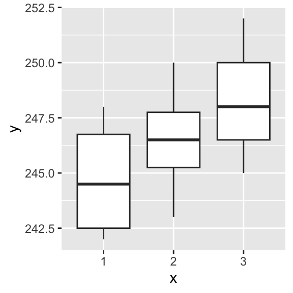

Using aov, \(Y\) is response, \(X\) is group.

fit.oneway.anova <- aov(y~x, data = coffee.data) 
summary(fit.oneway.anova)

##             Df Sum Sq Mean Sq F value  Pr(>F)   
## x            2   61.4  30.700   6.181 0.00616 **
## Residuals   27  134.1   4.967                   
## ---
## Signif. codes:  0 '***' 0.001 '**' 0.01 '*' 0.05 '.' 0.1 ' ' 1

anova(fit.oneway.anova)

## Analysis of Variance Table
## 
## Response: y
##           Df Sum Sq Mean Sq F value   Pr(>F)   
## x          2   61.4 30.7000  6.1812 0.006163 **
## Residuals 27  134.1  4.9667                    
## ---
## Signif. codes:  0 '***' 0.001 '**' 0.01 '*' 0.05 '.' 0.1 ' ' 1

model.tables(fit.oneway.anova, "means")

## Tables of means
## Grand mean
##       
## 246.5 
## 
##  x 
## x
##     1     2     3 
## 244.8 246.4 248.3

# plot(fit.oneway.anova) #diagnostic plots
coefficients(fit.oneway.anova)

## (Intercept)          x2          x3 
##       244.8         1.6         3.5

TukeyHSD(fit.oneway.anova, "x", ordered = TRUE)

##   Tukey multiple comparisons of means
##     95% family-wise confidence level
##     factor levels have been ordered
## 
## Fit: aov(formula = y ~ x, data = coffee.data)
## 
## $x
##     diff        lwr      upr     p adj
## 2-1  1.6 -0.8711391 4.071139 0.2606999
## 3-1  3.5  1.0288609 5.971139 0.0043753
## 3-2  1.9 -0.5711391 4.371139 0.1562593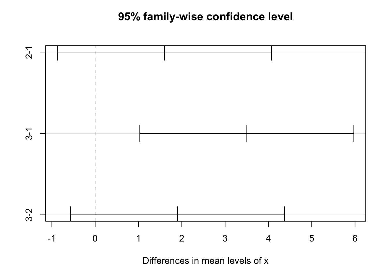

plot(TukeyHSD(fit.oneway.anova, "x"))

Using lm

fit.coffee <- lm(y~x, data = coffee.data)
summary(fit.coffee)

## 
## Call:
## lm(formula = y ~ x, data = coffee.data)
## 
## Residuals:
##    Min     1Q Median     3Q    Max 
## -3.400 -2.075 -0.300  1.675  3.700 
## 
## Coefficients:
##             Estimate Std. Error t value Pr(>|t|)    
## (Intercept) 244.8000     0.7047 347.359  < 2e-16 ***
## x2            1.6000     0.9967   1.605  0.12005    
## x3            3.5000     0.9967   3.512  0.00158 ** 
## ---
## Signif. codes:  0 '***' 0.001 '**' 0.01 '*' 0.05 '.' 0.1 ' ' 1
## 
## Residual standard error: 2.229 on 27 degrees of freedom
## Multiple R-squared:  0.3141, Adjusted R-squared:  0.2633 
## F-statistic: 6.181 on 2 and 27 DF,  p-value: 0.006163

anova(fit.coffee)

## Analysis of Variance Table
## 
## Response: y
##           Df Sum Sq Mean Sq F value   Pr(>F)   
## x          2   61.4 30.7000  6.1812 0.006163 **
## Residuals 27  134.1  4.9667                    
## ---
## Signif. codes:  0 '***' 0.001 '**' 0.01 '*' 0.05 '.' 0.1 ' ' 1

model.matrix(fit.coffee)

##    (Intercept) x2 x3
## 1            1  0  0
## 2            1  0  0
## 3            1  0  0
## 4            1  0  0
## 5            1  0  0
## 6            1  0  0
## 7            1  0  0
## 8            1  0  0
## 9            1  0  0
## 10           1  0  0
## 11           1  1  0
## 12           1  1  0
## 13           1  1  0
## 14           1  1  0
## 15           1  1  0
## 16           1  1  0
## 17           1  1  0
## 18           1  1  0
## 19           1  1  0
## 20           1  1  0
## 21           1  0  1
## 22           1  0  1
## 23           1  0  1
## 24           1  0  1
## 25           1  0  1
## 26           1  0  1
## 27           1  0  1
## 28           1  0  1
## 29           1  0  1
## 30           1  0  1
## attr(,"assign")
## [1] 0 1 1
## attr(,"contrasts")
## attr(,"contrasts")$x
## [1] "contr.treatment"

\(X_1\) is dropped. Compare ANOVA table with the 1-way ANOVA results.

Using lm with the constrain on the sum of effects equals 0.

options(contrasts=c('contr.sum', 'contr.sum'))
fit.coffee <- lm(y~x, data = coffee.data)
summary(fit.coffee)

## 
## Call:
## lm(formula = y ~ x, data = coffee.data)
## 
## Residuals:
##    Min     1Q Median     3Q    Max 
## -3.400 -2.075 -0.300  1.675  3.700 
## 
## Coefficients:
##             Estimate Std. Error t value Pr(>|t|)    
## (Intercept) 246.5000     0.4069 605.822  < 2e-16 ***
## x1           -1.7000     0.5754  -2.954  0.00642 ** 
## x2           -0.1000     0.5754  -0.174  0.86333    
## ---
## Signif. codes:  0 '***' 0.001 '**' 0.01 '*' 0.05 '.' 0.1 ' ' 1
## 
## Residual standard error: 2.229 on 27 degrees of freedom
## Multiple R-squared:  0.3141, Adjusted R-squared:  0.2633 
## F-statistic: 6.181 on 2 and 27 DF,  p-value: 0.006163

anova(fit.coffee)

## Analysis of Variance Table
## 
## Response: y
##           Df Sum Sq Mean Sq F value   Pr(>F)   
## x          2   61.4 30.7000  6.1812 0.006163 **
## Residuals 27  134.1  4.9667                    
## ---
## Signif. codes:  0 '***' 0.001 '**' 0.01 '*' 0.05 '.' 0.1 ' ' 1

model.matrix(fit.coffee)

##    (Intercept) x1 x2
## 1            1  1  0
## 2            1  1  0
## 3            1  1  0
## 4            1  1  0
## 5            1  1  0
## 6            1  1  0
## 7            1  1  0
## 8            1  1  0
## 9            1  1  0
## 10           1  1  0
## 11           1  0  1
## 12           1  0  1
## 13           1  0  1
## 14           1  0  1
## 15           1  0  1
## 16           1  0  1
## 17           1  0  1
## 18           1  0  1
## 19           1  0  1
## 20           1  0  1
## 21           1 -1 -1
## 22           1 -1 -1
## 23           1 -1 -1
## 24           1 -1 -1
## 25           1 -1 -1
## 26           1 -1 -1
## 27           1 -1 -1
## 28           1 -1 -1
## 29           1 -1 -1
## 30           1 -1 -1
## attr(,"assign")
## [1] 0 1 1
## attr(,"contrasts")
## attr(,"contrasts")$x
## [1] "contr.sum"

options(contrasts=c('contr.treatment', 'contr.treatment')) # to reset

Using lm, without intercept (this is the means model):

fit.coffee <- lm(y ~ x - 1, data = coffee.data)
summary(fit.coffee)

## 
## Call:
## lm(formula = y ~ x - 1, data = coffee.data)
## 
## Residuals:
##    Min     1Q Median     3Q    Max 
## -3.400 -2.075 -0.300  1.675  3.700 
## 
## Coefficients:
##    Estimate Std. Error t value Pr(>|t|)    
## x1 244.8000     0.7047   347.4   <2e-16 ***
## x2 246.4000     0.7047   349.6   <2e-16 ***
## x3 248.3000     0.7047   352.3   <2e-16 ***
## ---
## Signif. codes:  0 '***' 0.001 '**' 0.01 '*' 0.05 '.' 0.1 ' ' 1
## 
## Residual standard error: 2.229 on 27 degrees of freedom
## Multiple R-squared:  0.9999, Adjusted R-squared:  0.9999 
## F-statistic: 1.223e+05 on 3 and 27 DF,  p-value: < 2.2e-16

anova(fit.coffee)

## Analysis of Variance Table
## 
## Response: y
##           Df  Sum Sq Mean Sq F value    Pr(>F)    
## x          3 1822929  607643  122344 < 2.2e-16 ***
## Residuals 27     134       5                      
## ---
## Signif. codes:  0 '***' 0.001 '**' 0.01 '*' 0.05 '.' 0.1 ' ' 1

model.matrix(fit.coffee)

##    x1 x2 x3
## 1   1  0  0
## 2   1  0  0
## 3   1  0  0
## 4   1  0  0
## 5   1  0  0
## 6   1  0  0
## 7   1  0  0
## 8   1  0  0
## 9   1  0  0
## 10  1  0  0
## 11  0  1  0
## 12  0  1  0
## 13  0  1  0
## 14  0  1  0
## 15  0  1  0
## 16  0  1  0
## 17  0  1  0
## 18  0  1  0
## 19  0  1  0
## 20  0  1  0
## 21  0  0  1
## 22  0  0  1
## 23  0  0  1
## 24  0  0  1
## 25  0  0  1
## 26  0  0  1
## 27  0  0  1
## 28  0  0  1
## 29  0  0  1
## 30  0  0  1
## attr(,"assign")
## [1] 1 1 1
## attr(,"contrasts")
## attr(,"contrasts")$x
## [1] "contr.treatment"

1), 2) and 3) give the same ANOVA table. In 4), when the model does not include an intercept, the ANOVA table shows the uncorrected SS, i.e. \(\bar{y}\) not substracted:

SOURCE	df	SS
Regression	p	SSR
Error	n-p	SSE
Total	n	SST

Where \(SSR = \sum \hat{y}^2\), \(SSE = \sum(y - \hat{y})^{2}\) and \(SST = \sum y^{2}\).

It is also possible to fit the model by explicitly specifying the dummy variables.

# or using dummy variables

d1 <- as.numeric(coffee.data$x == 1)
d2 <- as.numeric(coffee.data$x == 2)
d3 <- as.numeric(coffee.data$x == 3)

fit.coffee.dummy <- lm(coffee.data$y ~ d1 +d2)
summary(fit.coffee.dummy)

## 
## Call:
## lm(formula = coffee.data$y ~ d1 + d2)
## 
## Residuals:
##    Min     1Q Median     3Q    Max 
## -3.400 -2.075 -0.300  1.675  3.700 
## 
## Coefficients:
##             Estimate Std. Error t value Pr(>|t|)    
## (Intercept) 248.3000     0.7047 352.326  < 2e-16 ***
## d1           -3.5000     0.9967  -3.512  0.00158 ** 
## d2           -1.9000     0.9967  -1.906  0.06730 .  
## ---
## Signif. codes:  0 '***' 0.001 '**' 0.01 '*' 0.05 '.' 0.1 ' ' 1
## 
## Residual standard error: 2.229 on 27 degrees of freedom
## Multiple R-squared:  0.3141, Adjusted R-squared:  0.2633 
## F-statistic: 6.181 on 2 and 27 DF,  p-value: 0.006163

#no intercept
fit.coffee.dummy2 <- lm(coffee.data$y ~ d1 +d2 +d3 - 1)
summary(fit.coffee.dummy2)

## 
## Call:
## lm(formula = coffee.data$y ~ d1 + d2 + d3 - 1)
## 
## Residuals:
##    Min     1Q Median     3Q    Max 
## -3.400 -2.075 -0.300  1.675  3.700 
## 
## Coefficients:
##    Estimate Std. Error t value Pr(>|t|)    
## d1 244.8000     0.7047   347.4   <2e-16 ***
## d2 246.4000     0.7047   349.6   <2e-16 ***
## d3 248.3000     0.7047   352.3   <2e-16 ***
## ---
## Signif. codes:  0 '***' 0.001 '**' 0.01 '*' 0.05 '.' 0.1 ' ' 1
## 
## Residual standard error: 2.229 on 27 degrees of freedom
## Multiple R-squared:  0.9999, Adjusted R-squared:  0.9999 
## F-statistic: 1.223e+05 on 3 and 27 DF,  p-value: < 2.2e-16

4.10 Confidence intervals and hypothesis tests for linear combinations of \(\boldsymbol{\beta}\)

From the theory of OLS:

\[\hat{\boldsymbol{\beta}} \sim N(\boldsymbol{\beta},(\mathbf{X}^T\mathbf{X})^{-1}\sigma^2)\]

and

\[\mathbf{c}^T\hat{\boldsymbol{\beta}} \sim N(\mathbf{c}^T\boldsymbol{\beta},\mathbf{c}^T(\mathbf{X}^T\mathbf{X})^{-1}\mathbf{c}\sigma^2)\]

For the caffeine example (1 way ANOVA model): suppose we want to compare the treatment means with the control mean, that is, we want a CI for:

\[\frac{\mu_2+\mu_3}{2}-\mu_1\]

Let \(\mathbf{c}^T= (-1, 1/2, 1/2)\), \(\boldsymbol{\beta}^T = (\mu_1, \mu_2, \mu_3)\).

\[\mathbf{c}^T\boldsymbol{\beta} = -\mu_1+\mu_2/2+ \mu_3/2\]

is estimated by:

\[\mathbf{c}^T\hat{\boldsymbol{\beta}} = -\bar{y}_{1.}+\bar{y}_{2.}/2+ \bar{y}_{3.}/2\]

and the variance is:

\[\begin{bmatrix} -1 & 1/2 & 1/2 \end{bmatrix} \frac{1}{10}\mathbf{I}_3 \begin{bmatrix} -1 \\ 1/2 \\ 1/2\end{bmatrix}\sigma^2 = \frac{3}{20}\sigma^2\]

So, the \(100 \times (1- \alpha) \%\)CI is:

\[\mathbf{c}^T\hat{\boldsymbol{\beta}} \pm t_{27}(\alpha/2) \sqrt{\frac{3}{20}\hat{\sigma}^2}\]

The df is: \(n-g = 30-3 = 27\).

We could also test hypotheses e.g. \(H_o: \mathbf{c}^T\boldsymbol{\beta} = 0\). The test statistic:

\[\frac{\mathbf{c}^T\hat{\boldsymbol{\beta}}}{\sqrt{\frac{3}{20}\hat{\sigma}^2}} \sim t_{27}.\]

3 Simple Linear regression

5 Model comparisons and testing for lack of fit