2 Introduction
2.1 Data and Models
Modeling: development of mathematical expressions that describe the behavior of a random variable of interest.
The variable of interest is called the response (or dependent) variable and denoted with \(Y\).
Predictor or explanatory variables (also called the independent variables) are thought to provide information on the behavior of \(Y\) and are incorporated into the model.
Predictor variables will be denoted as \(X\).
Data consist of information taken from \(n\) units. Subscripts \(i = 1,..., n\) identify the particular unit from which the observations were taken.
Additional subscripts can be used to identify different predictors.
All models involve unknown constants, called parameters, which control the behavior of the model. These parameters are denoted by Greek letters (e.g. \(\beta\)) and are to be estimated from the data.
We denote estimates using hat notation, e.g. \(\hat{\beta}\).
In this module we will study linear models. Here the parameters enter the model as simple coefficients on the \(X\)s or functions of \(X\)s.
2.2 Introductory Examples
A first look at how \(Y\) changes as \(X\) is varied is seen in a scatterplot.
2.2.1 Mother and daughter heights
Data from Pearson and Lee (1903).
heights <- read.table(here("data", "heights.txt"), header = TRUE)
head(heights)## Mheight Dheight
## 1 59.7 55.1
## 2 58.2 56.5
## 3 60.6 56.0
## 4 60.7 56.8
## 5 61.8 56.0
## 6 55.5 57.9- \(\bar{y}=\) 63.75, sd(\(y\)) = 2.6
heights |>
ggplot(aes(x = Dheight)) +
geom_histogram()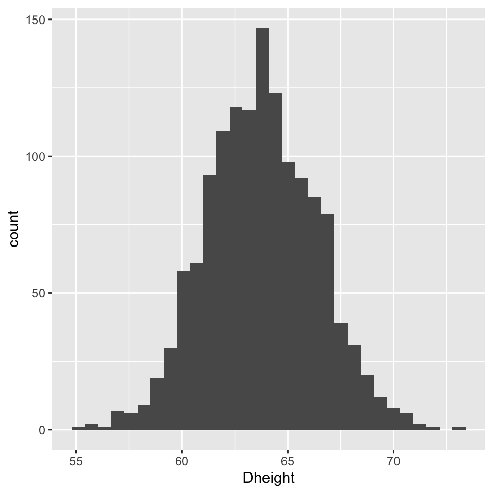
heights |>
ggplot(aes(x = Mheight, y = Dheight)) +
geom_point() +
geom_abline() +
xlab("mother height (inches)") +
ylab("daughter height (inches)")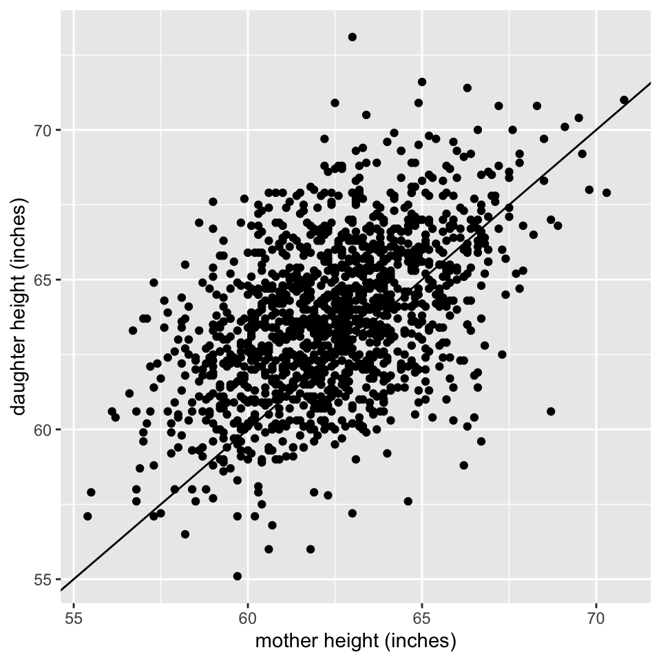
- Taller mothers have taller daughters.
- Since most points fall above line \(y=x\) most daughters are taller.
heights |>
ggplot(aes(x = Mheight, y = Dheight)) +
geom_point() +
geom_abline() +
geom_smooth(method = "lm", col = "red") +
xlab("mother height (inches)") +
ylab("daughter height (inches)")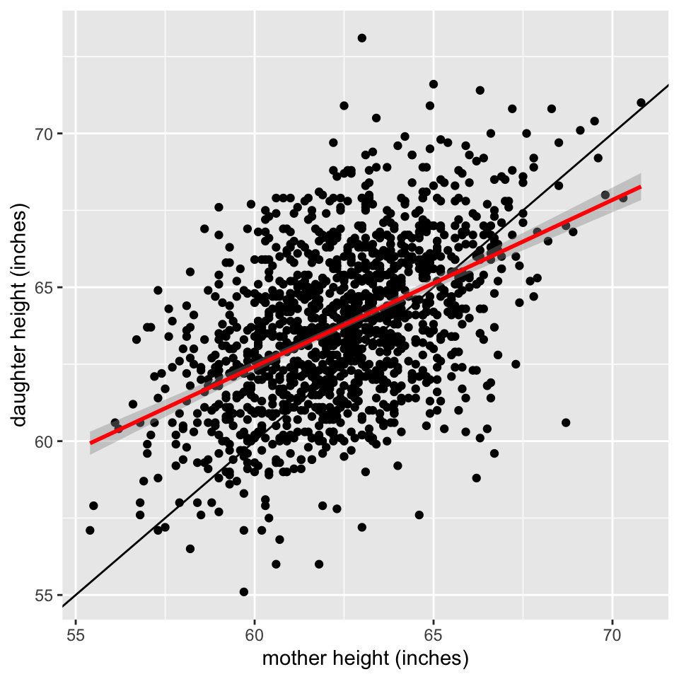
-Does the data follow a linear pattern? If so we can use the linear regression line to summarise the data.
-We can use the regression line to predict a daughters height based on her mother’s height.
- This is:
\(\hat{y}=\) 29.92 +0.54 \(x\)
2.2.2 Bacterial count and storage temperature
bacteria <- read.csv(here("data", "bacteria.csv"))

bacteria |>
ggplot(aes(x = temp, y = count)) +
geom_jitter(width = 0.1, height = .1) +
geom_smooth(method = lm, se = FALSE)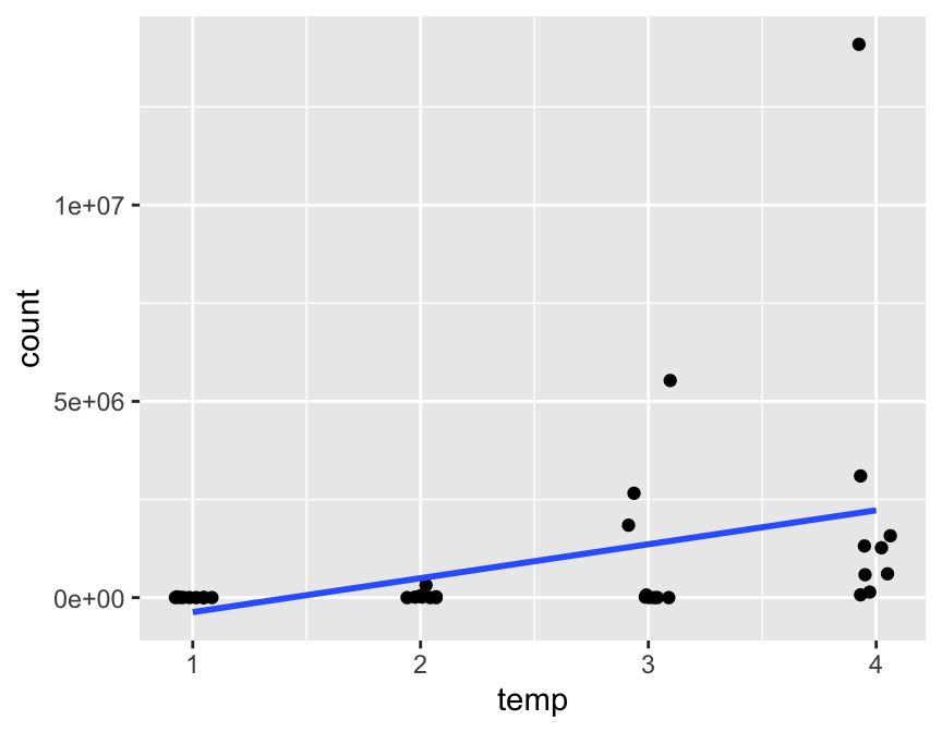
- Points are jittered to avoid overprinting.
- It does not appear to be a linear relationship.
- Consider a transformation?
bacteria |>
ggplot(aes(x = temp, y = log(count))) +
geom_jitter(width = 0.1, height = .1) +
geom_smooth(method = lm, se = FALSE)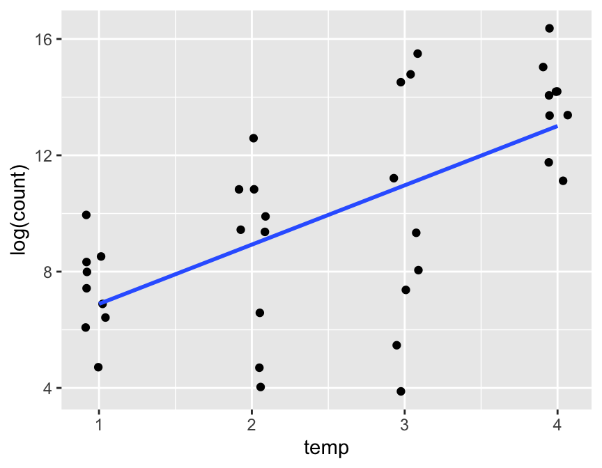
- Log transformed bacteria counts appear to have a linear relationship with temperature.
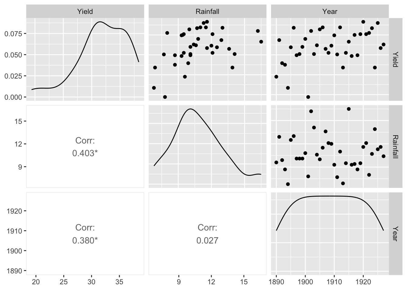
2.2.3 Yield and Rainfall
The dataset is from Ramsey and Schafer (2002). The data on corn yields and rainfall are in `ex0915’ in library(Sleuth3) (F. L. Ramsey et al. 2016). Variables:
- Yield: corn yield (bushels/acre)
- Rainfall: rainfall (inches/year)
- Year: year.
library(GGally)
library(Sleuth3)
ggpairs(ex0915[, c(2, 3, 1)], upper = list(
continuous = "points", combo = "facethist", discrete = "facetbar", na =
"na"
), lower = list(
continuous = "cor", combo = "box_no_facet", discrete = "count", na =
"na"
))
2.2.4 Driving
Example from: Weisberg (2005).
Study how fuel consumption varies over 50 US states and the District of Columbia and the effect of state gasoline tax on the consuption.
Variable:
- FuelC: Gasoline sold for road use, thousands of gallons
- Drivers:Number of licensed drivers in the state
- Income: Per person personal income for the year 2000, in thousands of dollars
- Miles: Miles of Federal-aid highway miles in the state
- Pop: 2001 population age 16 and over
- Tax: Gasoline state tax rate, cents per gallon
- State: State name
We will use a scatterplot matrix.
driving <- read.table(here("data", "fuel2001.txt"), header = TRUE)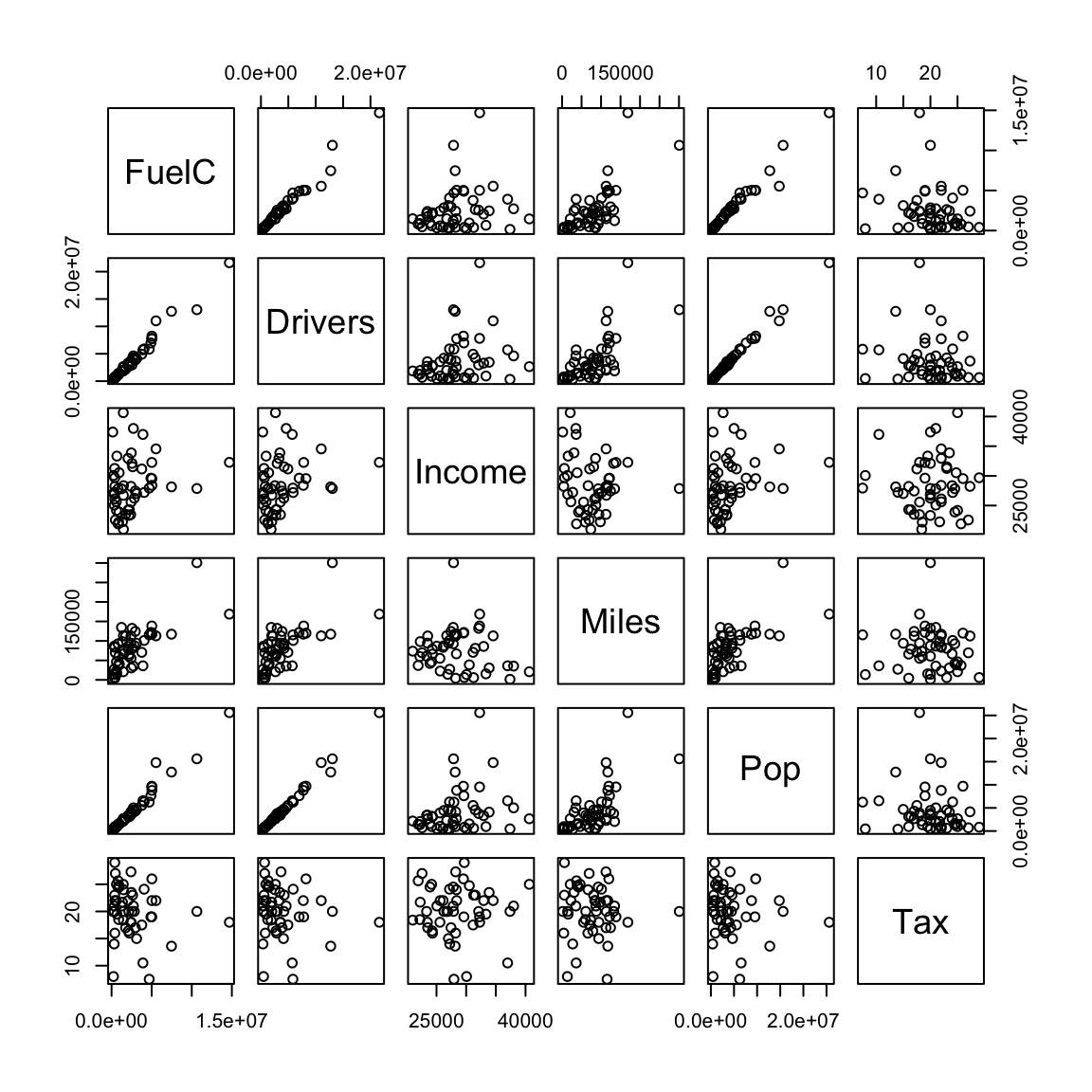
- Both Drivers and FuelC are state totals so will be larger in more populous states.
- Income is per person, we want to make variables comparable.
Transform variables:
- FuelC2:FuelC/Pop
- Drivers2: Drivers/Pop
- Miles2:log\(_2\)(Miles)
driving2 <- driving |>
mutate(Drivers = Drivers / Pop,
FuelC = FuelC / Pop,
Miles = log(Miles, 2))


pairs(driving2[, c(2, 1, 3, 4, 5, 6)])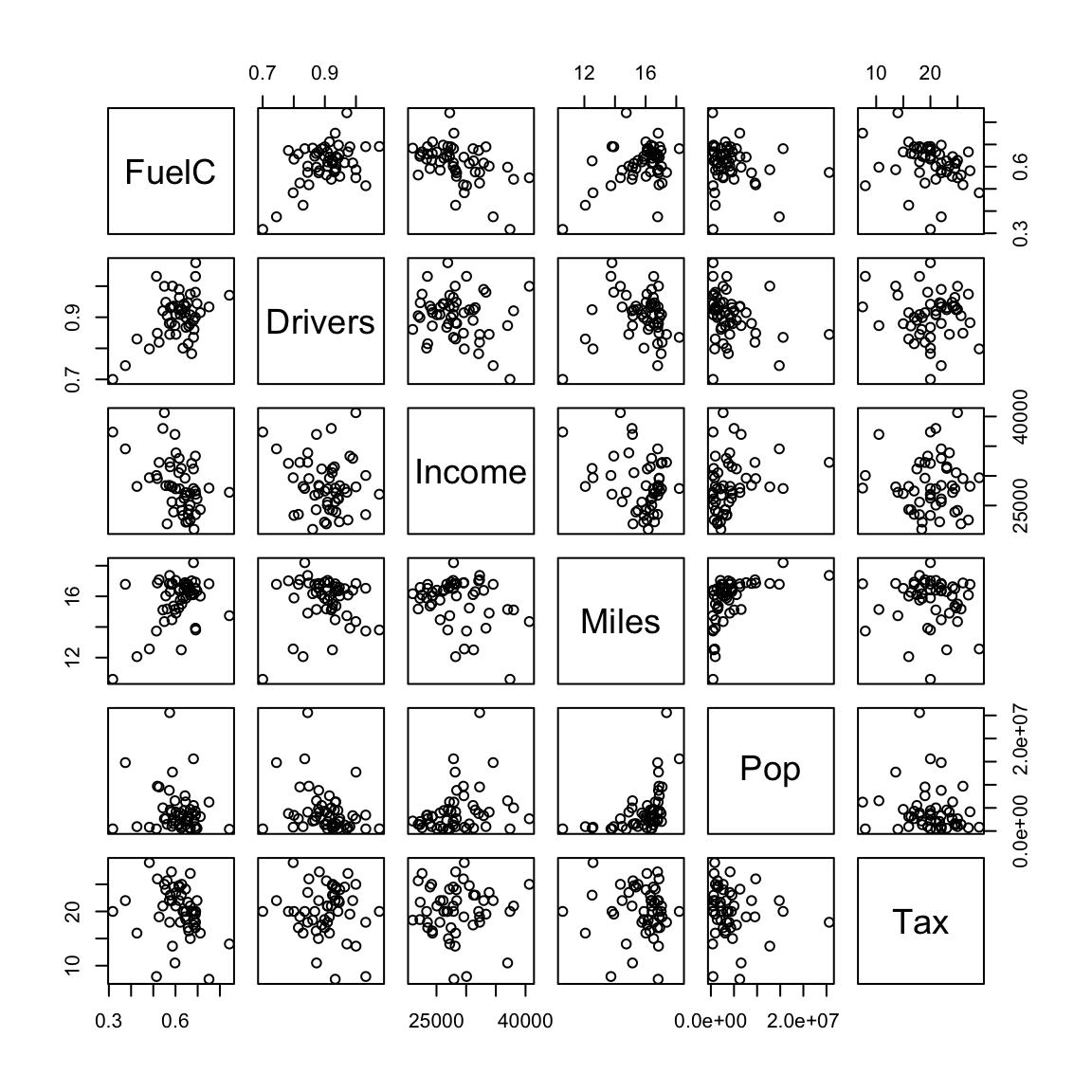
- FuelC decreases as tax increases but there is a lot of variation.
- Fuel is weakly related to a number of other variables.
Other graphical representations of the dataset:
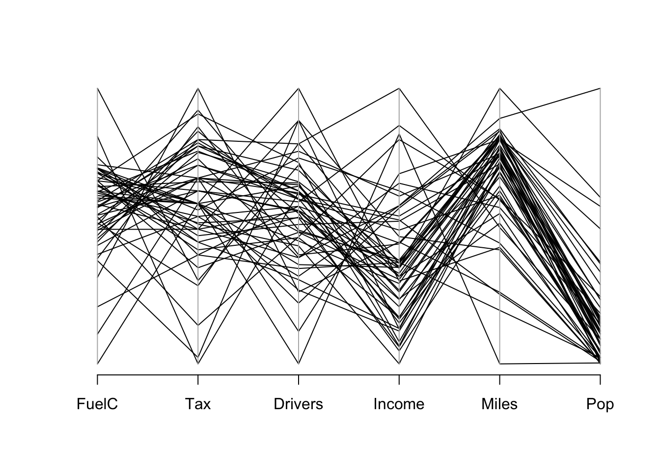 Parallel coordinates in package
 MASS (Venables and Ripley 2002).
We can fit a linear model predicting FuelC using all other variables. We would be particularly interested in the relationship between Tax and FuelC but we need to take into account (adjust for) the other predictors.
We can also look at the data and the model that we will fit using conditional visualisation (C. B. Hurley, O’Connell, and Domijan 2022) in R package condvis2 (C. Hurley, OConnell, and Domijan 2022). If you run the code below, it will open an interactive plot in a separate window. It shows a low-dimensional visualisation, constructed showing the relationship between the response FuelC and the predictor Tax, conditional on the remaining predictors. The conditioning values can be selected within the shiny app.
2.2.5 Fuel Consumption
Information was recorded on fuel usage and average temperature (\(^oF\)) over the course of one week for eight office complexes of similar size. Data from Bowerman and Schafer (1990).
We expect fuel use to be driven by weather conditions.
Fuel use: response or dependent variable. Denoted by \(Y\).
Temperature: Explanatory or predictor variable. Denoted by \(X\).
We observe n=8 pairs: \((x_{i}, y_{i}), i =1,...,8\).
Temp <- c(28, 28, 32.5, 39, 45.9, 57.8, 58.1, 62.5)
Fuel <- c(12.4, 11.7, 12.4, 10.8, 9.4, 9.5, 8, 7.5)

FuelTempData <- data.frame(cbind(Temp, Fuel))| Temp | Fuel |
|---|---|
| 28.0 | 12.4 |
| 28.0 | 11.7 |
| 32.5 | 12.4 |
| 39.0 | 10.8 |
| 45.9 | 9.4 |
| 57.8 | 9.5 |
| 58.1 | 8.0 |
| 62.5 | 7.5 |
FuelTempData |>
ggplot(aes(x = Temp, y = Fuel)) +
geom_point() +
geom_smooth(method = lm, se = FALSE)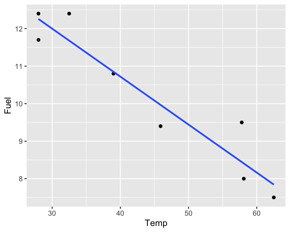
The scatterplot shows that fuel use decreases roughly linearly as temperature increases.
We assume there’s an underlying true line: \[\mbox{Fuel} =\beta_{0} + \beta_{1}\mbox{Temp} + \epsilon\]
or, more generally: \(y =\beta_{0} + \beta_{1}x + \epsilon.\)
The intercept (\(\beta_0\)) and slope (\(\beta_1\)), are unknown parameters and \(\epsilon\) is the random error component.
For each observation we have:\(y_i =\beta_{0} + \beta_{1}x_i + \epsilon_i\).
We can estimate \(\beta_0\) and \(\beta_1\) from the available data.
One method that can be used to do this is the method of ordinary least squares.
NOTE: other models are possible:
FuelTempData |>
ggplot(aes(x = Temp, y = Fuel)) +
geom_point() +
geom_smooth(method = loess, se = FALSE)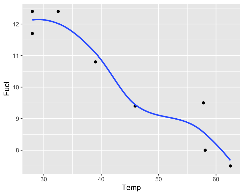
2.2.6 Elections and Economy

Variables:
- year: 1952 to 2012
- growth: inflation-adjusted growth in average personal income
- vote: percentage of votes for the incumbent party’s candidate in US presidential elections
The better the economy was performing, the better the incumbent party’s candidate did, with the biggest exceptions being 1952 (Korean War) and 1968 (Vietnam War).
Example from (Gelman, Hill, and Vehtari 2020) available in package (Gelman, Hill, and Vehtari 2025).